
Data Storage & Management for Image AI Pipelines
A Data-Centric View of Image AI Pipelines
This page presents the "Data Storage and Management for Image AI Pipelines" tutorial, which was published and presented at SIGMOD 2025. The tutorial aims to present a data-centric view of image AI pipelines by combining cross-disciplinary materials from digital signal processing, computer vision, and computer systems into a unified view of data management systems. It assumes no prior knowledge of AI or machine learning. Its audience is PhD students, professors, researchers, and entrepreneurs.
Are you interested in? Send us an email.

Image AI Pipelines are Data Management Pipelines
Image AI Improves Every Aspect of Modern Human Life. Image AI has shown great success in numerous areas, providing more productive and safer services and tools. Medical doctors now use image AI to support their decision-making process in the early and late detection of diseases. Companies deploy image AItools to enhance worker safety conditions. Manufacturing companies use image AI in their production pipelines to increase productivity. Farmers use image AI to efficiently monitor the conditions of their crops and take preventive actions against potential diseases, further improving their yields.
Image AI is Expensive. Every year, billions of digital cameras capture trillions of images. These images consume thousands of petabytes of storage in the cloud. Numerous AI applications process these massive datasets for various purposes, such as personalized content management, image reconstruction, and visual captioning. Applications access data over remote storage servers and need to move and process data in compute nodes using high-end processors. This incurs an immense dollar cost for cloud vendors and application developers. It costs millions of dollars to train and deploy a single model, which generates hundreds of thousands of pounds of carbon emissions, making image AI inaccessible.
Image AI Pipeline. A typical image AI pipeline is composed of four main operations. The first one is fetching raw data from persistent storage, which can be remote, local, or a combination of the two.The second is converting raw data into a learnable in-memory format, such as the visually recognizable red-green-blue (RGB) format. Today, CPUs primarily perform this conversion. Third, the learnable format of images from the host memory moves to one or more GPU devices. GPUs primarily run image AI models in a single or multi-GPU setting, depending on the AI model’s size and data. This movement typically happens over a device-to-device connection such as PCIe or a fast interconnect network providing fast direct communication across devices within the same server. Lastly, the AI models process the moved images in their learnable formats to perform the particular AI task, such as training the AI model or performing inference over the images using the AI model residing on the GPU.
Data Management is Key for Efficient Image AI. The cost of these operations is fundamentally defined by how efficiently image AI systems manage their data. Fetching and storing image data are defined by the storage/file formats used for images. While some algorithms aggressively compress images, some lightly compress, each leaving an image AI pipeline with different trade-offs. Converting raw image data into a learnable format and how and when the conversion happens is defined by the storage format used. While standard storage formats use visually recognizable RGB format, recent AI-task-specific formats use semi-compressed visually unrecognizable formats for a more efficient decoding process. Moving images from host memory to the GPU memory depends on how images are represented in main memory, as well as available GPU memory consumed by multiple parties such as the AI model itself as well as the batches of images and gradients. Efficient management of data objects within and across host-to-GPU memory is crucial to fit large models into GPUs and train them efficiently. Similarly, performing an AI task within a GPU requires efficiently handling data objects of the AI model itself together with the gradients and batches of images, including compressing them efficiently, swapping them back-and-forth GPU memory, and executing multiple AI models or multiple data batches in parallel to improveGPU utilization. From raw data to execution of AI models, managing data plays a key role in making image AI systems efficient.
Tutorial Structure. This tutorial presents a data-centric view of image AI pipelines by combining cross-disciplinary materials from digital signal processing, computer vision, and computer systems into a unified view of data management systems. The figure above presents the tutorial’s structure over an image AI pipeline. It is composed of five sections. The first section provides essential background information on the main algorithm used for training image AI models: Gradient Descent. The second to fifth sections cover how image AI pipelines manage the four main data objects that they produce and consume: (1) Images, (2) Activations, (2) Gradients, and (4) Parameters. Images stand for the image data used for training and inference of AI models. Activations and Gradients are intermediate data objects produced and consumed by AI models. Parameters refer to the AI model parameters, which constitute a major bottleneck for large models. Lastly, section six will present an overview and list open problems. At the end of each section, a reading list is provided that points to relevant papers.


Section 1. Background: Gradient Descent
Gradient Descent is an optimization algorithm used to minimize the value of an objective function. The figure below illustrates the high-level algorithm. Suppose we have an objective function that maps the value of a parameter (weight, on the x-axis) to a corresponding cost value (y-axis). Gradient Descent allows finding the optimum weight value with the minimum cost. It achieves this by starting with a random weight value (shown as the black point on the figure below). It then takes the derivative of the objective function with respect to the weight. Derivative of the objective function is simply another function. Gradient Descent substitutes the starting weight value into the derivative of the objective function and uses the resulting value to update the starting weight value (also shown by the right-hand side of the figure below).

Its motivation is as follows. The derivative of the objective function at a specific point (in this case, the starting weight value) defines how the objective function changes at that point. This is the definition of derivative. It defines the rate of change. If the derivative is high, it means the function is increasing or decreasing steeply. If the derivative is low, it means the function is rather flat. Gradient Descent subtracts the derivative from the starting weight value. It subtracts rather than adds. The reason is again related to the definition of derivative. Derivative defines not only the magnitude of the rate of change, but also the direction of the rate of change. If the derivative is positive, it means the function is increasing at that point. If the derivative is negative, it means the function is decreasing at the point. As our goal is to minimize the objective function, Gradient Descent subtracts the derivative value from the initial weight value, as also shown on the right-hand side of the figure above.
The last element in Gradient Descent is the parameter known as the learning rate, denoted by lr in the figure above. It is used to scale the derivative value. A high learning rate can accelerate learning, but it can also cause zigzags in the optimization process. A low learning rate could provide more stable learning, but it could also get stuck in a suboptimal region in the optimization space and/or take a long time to complete. Once the starting weight value is updated by using the derivative of the objective function, Gradient Descent iterates over the same process with the new weight value, ultimately reaching a minimum objective value.
Most AI models are trained by using a version of the Gradient Descent algorithm. Achieving this requires first casting the learning problem as an optimization problem. Learning algorithms define a loss function that computes the difference between the AI model's predicted outcome and the real outcome. This loss function is used as the objective function, which Gradient Descent optimizes by taking derivatives of the loss function and incrementally updating AI model parameters. The loss function is computed using two key ingredients: the AI model parameters and the input data. At every iteration of Gradient Descent, AI model parameters are updated such that the loss function is optimized to have a minimal "loss" value. There are three important definitions here: (i) partial derivatives, (ii) forward pass, and (iii) backward pass.
The partial derivative of a function defines the derivative of a function with respect to a particular variable. AI models contain a large number of parameters. Hence, when optimizing the loss function, it is necessary to analyze each parameter individually, which requires calculating the partial derivatives of the loss function for every single parameter of the AI model. The vector of all partial derivatives of a function is called the gradient of the function; hence comes the name of the Gradient Descent. When training an AI model, the gradients of the loss function are iteratively computed and applied to all the model's parameters, as briefly described in the figure above.
The forward pass defines a single pass over the AI model to compute the loss function for a single step of Gradient Descent. As shown in the figure above, modern AI models consist of multiple layers. Every layer produces and consumes a set of data objects successively, which eventually leads to computing probabilities that define the AI model's prediction. The backward pass defines the computation of gradients for all model parameters. Gradient computation proceeds from the last to the first layers due to the use of a specific rule when taking the partial derivative of the loss function: the Chain Rule. The chain rule enables the differentiation of complex functions. As AI models are composed of multiple layers and hence are complex mathematical functions, the chain rule is necessary to compute their gradients. The chain rule operates in a backward fashion, starting from the last layer of the model and working its way back to the first layer of the model. Once gradient computations are finished, the AI model parameters are all updated at once, completing a single step of Gradient Descent.
An inference in this context refers to a single forward pass, where the AI model performs predictions without computing the loss function. A training step refers to a forward and backward pass. The forward pass computes the loss function, and the backward pass computes the gradients, updating the model parameters based on these gradients.


Section 2. Data Object #1: Images
Images are the first data object that image AI pipelines consume. They are responsible for the time and resources consumed at every level in the image AI pipeline, from disk/network I/O to the GPU. In the figure below, we profile end-to-end image AI inference time using a popular AI model, MobileNet V3. We quantify how much time it takes to read the images from the disk as JPEG files (Disk I/O component), how much it takes to convert images into a visual format (CPU component), how much it takes to transfer images from CPU to GPU (Transfer component), and how much time it takes to run the AI model over the images on the GPU (GPU component). As the figure shows, 90% of the time is spent on non-GPU tasks, which primarily involve reading images from the disk, converting them into a visual format, and then transferring them from the CPU to the GPU.

All these time components depend on how images, as data objects, are stored on disk and represented in main memory. Disk and CPU times depend on the storage algorithm. Transfer and GPU times depend on how images are represented in main memory. A high-resolution image with a large spatial dimension has a significantly different transfer and GPU time than a low-resolution image. In this section, we cover major image AI storage formats that define how images are stored and represented in main memory.
2.1 Standard Formats

Most images are today stored as JPEG files. The Joint Photographic Experts Group developed JPEG, and it is a multi-stage compression algorithm that incorporates both lossy and lossless compression steps. It minimizes stored data by discarding information without significantly compromising visual quality. The figure above presents JPEG's writing (top row) and reading (bottom row) algorithms. When storing an image, JPEG first subsamples the image into a lower spatial dimension. It subsamples only color components, as these have a relatively lower impact on visual quality compared to other elements, such as brightness. It then partitions the image into blocks and transforms each block from the pixel-based color domain into the so-called frequency domain.
Every value in the frequency domain represents a coefficient for a specific signal with a particular frequency. A signal is simply an array of values that can be considered as flowing over time. A low-frequency signal is a signal whose values change slowly over time. A high-frequency signal is a signal whose values frequently change. JPEG performs frequency transformation, as it is known that visual quality is primarily defined by low-frequency information rather than high-frequency information. Hence, when storing images, JPEG more aggressively compresses high-frequency information than it does for low-frequency information, which allows a better trade-off in terms of losing visual quality versus on-disk storage. Once JPEG compresses high-frequency information, it uses an entropy coding technique to encode the frequency coefficients into a file for storage on disk or transmission over the network. Reading an image, i.e., reconstructing an image, is simply the reverse of storing it. It decodes the coefficients from the disk.
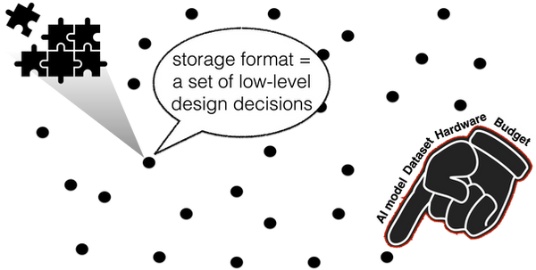
JPEG is designed for digital photography. Its goal is to lossily compress images without losing much visual quality. AI problems, however, are diverse. Every image AI problem has unique characteristics regarding how data should be stored and processed. We define an AI problem as a quadruple: dataset, AI model, machine, and performance budget. Any change in any dimension of an AI problem creates an entirely new problem and requires a re-design of the storage. For example, a storage with five milliseconds of inference budget could be completely different than a storage with a hundred milliseconds of inference budget. Therefore, using a fixed design for all problems is inefficient and can lead to severe performance issues due to excessive data movement.
Researchers have realized this problem and proposed several alternatives to JPEG, or any standard storage format. Main idea is to create a new, tailored storage format for a given AI problem. The following two sections cover two such methods: (i) self-designed storage format, and (ii) learned storage formats. Self-designed formats define a design space of storage formats within which they search for the optimal one for a given AI problem. Learned formats cast this problem as a learning problem and uses popular autoencoder neural architectures to learn a representation that is tailored to the AI problem.
Reading List:
[1] https://en.wikipedia.org/wiki/JPEG
[2] G.K. Wallace. 1992. The JPEG Still Picture Compression Standard. IEEE Transactions on Consumer Electronics 1992.
2.2 Self-Designed Formats
A self-designed format defines a design space of storage formats and a search algorithm used to search within this design space with a specific goal. Every candidate in the design space represents a distinct storage format, characterized by a unique trade-off between inference, training time, storage, and accuracy. Accuracy refers to precision of the AI model, e.g., image classification accuracy. Formats with a small storage and high inference/training time usually offers a lower accuracy, and vice versa. Goal of a self-designed format is find the format that maximizes accuracy and minimizes the cost, for a specific AI problem and cost budget.
Design Space. Creating a design space of storage formats requires breaking down image storage formats and understanding their main design primitives. A rich design space encompasses a large number of candidates, each offering a distinct trade-off between space, inference/training time, and accuracy. There are four main design primitives cover all standard storage formats: (i) Sampling, (ii) Partitioning, (iii) Pruning, and (iv) Quantization. Sampling defines removing a set of columns and/or rows from the image. Partitioning refers to decomposing an image into blocks and storing or reading them block by block rather than as a whole image. Pruning refers to the removal of unnecessary data from the image. Quantization refers to reducing the magnitude of the values in image data so that they can be encoded with a smaller number of bits. These four primitives govern all canonical storage formats. JPEG in its default settings, for example, samples images at every other row and column, partitions them into 8x8 blocks, and uses a specific 8x8 quantization matrix to quantize every data value within the block with a specific quantization factor. Learned JPEG, on the other hand, in addition to performing the same sampling, partitioning, and quantization as standard JPEG, also prunes unuseful data based on a learned model defining which data items are useful and which are not. Video storage formats follow image storage formats, except that they use sophisticated algorithms for exploiting the temporal relationship within the video data. They, too, use similar primitives, such as partitioning, sampling, and quantization when storing data.
Domains for Design Primitives. Design primitives define the fundamentals when storing images. They are, however, useful only when we know how to perform each design primitive. A domain defines the set of possible ways to perform a specific design primitive. Every design primitive has its domain. Every combination of every domain value across all design primitives defines a different storage format, and all such combinations collectively define the total design space. There are, however, exponentially many ways to perform each design primitive. An RGB image, for example, can be sampled in an exponentially large number of ways. Similarly, we can partition the image into blocks of any size and prune them in an exponentially large number of ways.Consider a block size of 8x8, i.e., images are partitioned into 8x8 blocks when storing, and assume that we apply the same pruning strategy to all blocks of the image. How many possible pruning strategies are therefor, say, six different block sizes: 8x8,16x16, 32x32, ..., 256x256? For8x8 block size, there are 2^{8x8} = 2^64 possible pruning strategies. For 16x16 blocks, there are 2^{16x16} = 2^256 strategies. In total, this makes 2^{8x8} + 2^{16x16} + ... + 2^{256x256} > 10^150K, which is beyond any computational capacity to search within.
Dimensionality Reduction. Self-designed formats use sensitivity analyses for each design primitive to determine a feasible domain. Their goal is to reach conclusions for each design primitive such that certain values of their domains perform significantly better than others. This way, they aim to determine the most valuable set of design decisions for each primitive and create a feasible yet high-quality design space. When performing the sensitivity analysis, they fix values of all design primitives except the primitive under test. They then vary the values of the primitive under test from a very small value to a very large value and analyze how various AI problems, using different datasets and AI models, perform across different ranges of values. If they identify a group of domain values that are worse than others, they exclude them from the domain. If all domain values perform similarly, they uniformly sample a feasible set of domain values. This way, they identify the most valuable design decisions for each design primitive and create a high-quality design space.
Design Space: ~4K Storage Formats. Having defined the domains, the total number of elements in the design space is ~4K. There are three quantization factors, four sampling strategies, six block sizes, and as many pruning strategies as the dimension of each block size. This variation in total sums up to 4104 storage formats, which is large yet feasible enough to search within.
Search. Design space constitutes the core of a self-designed format. It defines the boundaries of the quality and efficiency that a self-designed format offers. In terms of the search algorithm, any search algorithm could be used. There are two main lines of search algorithms: (i) trial-and-error-based, and (ii) self-supervised. Trial-and-error-based algorithms perform a search similar to that of neural architecture or hyperparameter search, where they train an AI model for every candidate storage format for a small number of epochs and converge on a specific candidate over iterations. Transfer-learning-based weight-sharing methods are examples of this. Self-supervised search algorithms learn an embedding for each candidate in the design space and use locality among candidates in the learned embedding space to search efficiently.
Reading List.
[1] The Image Calculator: 10x Faster Image-AI Inference by Replacing JPEG with Self-designing Storage Format. Utku Sirin, Stratos Idreos. SIGMOD, 2024.
[2] Frequency-Store: Scaling Image AI by A Column-Store for Images. Utku Sirin, Victoria Kauffman, Aadit Saluja, Florian Klein, Jeremy Hsu, Stratos Idreos. CIDR, 2025.
[3] Scalable Image AI via Self-Designing Storage. Utku Sirin, Victoria Kauffman, Aadit Saluja, Florian Klein, Jeremy Hsu, Vlad Cainamisir, Qitong Wang, Konstantinos Kopsinis, Stratos Idreos. IEEE Data Engineering Bulletin, 2025.
More Readings for Neural Architecture and Hyper-parameter Search:
[4] DARTS: Differentiable Architecture Search. Hanxiao Liu, Karen Simonyan, Yiming Yang. ICLR 2019.
[5] AutoHAS: Differentiable Hyper-parameter and Architecture Search. Xuanyi Dong, Mingxing Tan, Adams Wei Yu, Daiyi Peng, Bogdan Gabrys, Quoc V. Le. arXiv, 2020. https://arxiv.org/pdf/2006.03656v1
[6] AutoHAS: Efficient Hyperparameter and Architecture Search. Xuanyi Dong, Mingxing Tan, Adams Wei Yu, Daiyi Peng, Bogdan Gabrys, Quoc V. Le. ICLR 2021, Workshop on Neural Architecture Search.
[7] BOHB: Robust and Efficient Hyperparameter Optimization at Scale. Stefan Falkner, Aaron Klein, Frank Hutter. ICML 2018.
[8] BANANAS: Bayesian Optimization with Neural Architectures for Neural Architecture Search. Colin White, Willie Neiswanger, Yash Savani. AAAI 2021.
2.3. Learned Formats

Learned formats utilize the popular autoencoder neural network architecture to discover a data representation tailored to the specific AI task. Autoencoder architectures use an encoder and a decoder block to encode images into an intermediate data representation, which the decoder block learns to accurately reconstruct the original images. An intermediate data representation is simply a matrix of floating-point or integer values. The encoder or decoder block is simply a neural architecture block that performs computations over the images or the learned intermediate data representation. Learning is accomplished by minimizing a loss function that computes the difference between the reconstructed and original image.
Task-specific learned formats follow the same idea, except that they replace the decoder block with a neural architecture block that performs the AI task. To illustrate, if it is an image classification task, the task-specific block learns to map the intermediate data representation to a specific image-class, e.g., a dog. This way, task-specific encoding learns an intermediate data representation that is tailored to the given AI task.
Self-Designed versus Task-Specific Learned Formats. Task-specific learned formats use the power of latent-space reasoning, which means they encode a matrix of floating point values fine-tuned for the given task. Compared to self-designed formats, this could achieve a higher quality due to working on a much larger search space. However, the size of the search space also complicates the learning problem and can unpredictably lead to failure for different AI tasks. Furthermore, it requires learning a new representation for every AI task, for every cost budget again and again, whereas self-designed formats rely on a well-designed designed design space shown to work across various domains and tasks. Lastly, self-designed formats rely on a well-defined design primitives, which allows reasoning about the candidates in its design space and provides explainability in deciding on which storage format to use and even improving existing storage formats. Learned formats merely allow trying yet another neural architecture in hoping that it could potentially provide a higher quality data representation. Lastly, learned formats' intermediate data representation is often of fixed size, e.g., a 64x64 matrix. This dimension should change for every cost budget, making the search problem even costlier.
Reading List:
[1] Reducing the Dimensionality of Data with Neural Networks. G. E. Hinton and R. R. Salakhutdinov. Science 2006.
[2] End-to-end Optimization of Nonlinear Transform Codes for Perceptual Quality. Johannes Ballé, Valero Laparra, Eero P. Simoncelli. PCS 2016.
[3] End-to-end Optimized Image Compression. Johannes Ballé, Valero Laparra, Eero P. Simoncelli. ICLR 2017.
[4] End-to-End Image Classification and Compression With Variational Autoencoders. Lahiru D. Chamain, Siyu Qi, and Zhi Ding. IEEE Internet of Things Journal 2022.
[5] Deep Feature Compression for Collaborative Object Detection. Hyomin Choi and Ivan V. Bajić. ICIP 2018.
[6] Learning in Compressed Domain for Faster Machine Vision Tasks. Jinming Liu, Heming Sun, and Jiro Katto. VCIP 2021.
[7] Learning From the CNN-based Compressed Domain. Zhenzhen Wang, Minghai Qin, and Yen-Kuang Chen. WACV 2022.
[8] Learning in the Frequency Domain. Kai Xu, Minghai Qin, Fei Sun, Yuhao Wang, Yen-Kuang Chen, Fengbo Ren. CVPR 2020.

Section 3. Data Object #2: Activations
Images as a data object constitute the major bottleneck in image AI pipelines, as they determine the amount of data moved and processed throughout the entire pipeline. However, once an AI model starts processing images, there are multiple large data objects other the images themselves that cause as significant problems as images. First one of these objects are activations, also called activation maps, or feature maps. These are intermediate data objects that an AI model produces while it processes a batch of images.
Modern AI models are layered. At every layer, an AI model consumes the data object produced by the preceding layer, and it creates a new data object that the subsequent layer will consume. These intermediate data objects are referred to as activations, as also illustrated in the figure above. These activations are massive data objects, as they store all the intermediate features that the AI model learns through an extensive amount of neural computations. For a single image, a typical AI model produces an activation that is hundreds of times bigger than the image in a single layer. Once accumulated over a large number of layers, activations constitute a major memory bottleneck for training large AI models. Given that GPUs have a limited amount of memory, activations often limit the size of the AI model that a single GPU can train, which further limits the precision of the achieved task.
Activations are Necessary for Computing Gradients. A natural question to ask is "Why can't we simply discard a computed activation once a layer has consumed it and produced the next activation?". We can, but only for inference. As explained in the background section, inference requires a single forward pass over the AI model. During the forward pass, it is indeed that AI models keep two activations at a time, the input and output activations for the active layer that performs the processing. For training, however, both forward and backward passes are necessary. While forward pass produces activations, backward pass uses those activations to compute gradients. This is because modern AI models are trained by using the Gradient Descent algorithm, which is briefly explained in the first section. Gradient Descent requires an objective function to minimize by using derivatives. The objective function for an AI model is the function that defines the difference between the predicted and actual outcomes, as its goal, i.e., the objective, is to make predictions that are as close to the actual outcomes as possible. Learning algorithms achieve this by using a "loss function" that computes the difference between the actual and predicted outcomes. Gradient Descent uses gradients, i.e., a vector of partial derivatives of the loss function, to incrementally update the parameters of the AI model, such that the updated parameters reduce the loss at every single training step, as explained in the background section. Activations are necessary for computing the gradients. Every partial derivative requires a specific activation. Hence, learning algorithms maintain costly activations until they are used to compute a specific partial derivative in the loss function. Once a partial derivate is computed, its dependent activations can be released from the GPU memory.
Materialize to CPU Memory or Discard & Recompute. Learning systems use two primary methods to reduce memory pressure caused by the activations: (i) Materialize & Reuse, (ii) Discard & Recompute. The Materialize & Reuse method leverages large CPU DRAM into the learning process. Today's commodity servers are equipped with large main memories, ranging from hundreds of gigabytes to several terabytes of capacity. Hence, once computed, learning systems materialize activations into the CPU memory, i.e., they transfer activations from the GPU memory to the CPU memory and retain them there until it is necessary to compute a specific partial derivative. Once required, learning systems swap the activation back into GPU memory, compute the relevant gradient, and then release the GPU memory occupied by the activation. This way, learning systems significantly reduce the GPU memory pressure caused by activations, allowing for the training of large AI models on a single GPU.
The Discard & Recompute method discards the activations as soon as they are consumed by the layer processing them, instead of swapping them to CPU memory. Once needed, learning systems recompute the activation by running the entire computation from scratch to compute the specific activation required to compute the particular gradient. While this method could be costlier than swapping back and forth between CPU and GPU memory, it might allow faster training under certain circumstances, such as when the transfer time between CPU and GPU is very high.
Reading List:
[1] Capuchin: Tensor-based GPU Memory Management for Deep Learning. Xuan Peng, Xuanhua Shi, Hulin Dai, Hai Jin, Weiliang Ma, Qian Xiong, Fan Yang, and Xuehai Qian. ASPLOS 2020.
[2] Checkmate: Breaking the MemoryWall with Optimal Tensor Rematerialization. Paras Jain, Ajay Jain, Aniruddha Nrusimha, Amir Gholami, Pieter Abbeel, JosephGonzalez, Kurt Keutzer, and Ion Stoica. MLSys 2020.
[3] mu-TWO: 3x Faster Multi-Model Training with Orchestration and Memory Optimization. Sanket Purandare, Abdul Wasay, Animesh Jain, and Stratos Idreos. MLSys 2020.


Section 4. Data Object #3: Gradients
As explained in the background section, the gradient of a function is a vector of partial derivatives. There are as many partial derivatives as the number of variables of the function. Hence, for an AI model, there is one partial derivative for every parameter. The total number of partial derivatives equals the number of parameters in the AI model. As shown in the previous section on activations, gradients do not pose a significant memory bottleneck, especially for models that can fit into a single GPU. They do, however, pose a considerable challenge in terms of the communication bottleneck.

Data-Parallel Execution. Most AI models today are trained using data-parallel execution. Data-parallel execution samples multiple batches of images and trains a separate copy of the AI model on multiple GPUs in parallel, as also shown in the figure above. This significantly accelerates training, especially for large datasets. Data-parallel execution requires communicating gradients across GPUs to synchronize the parameters of multiple copies of the AI model. Communication cost is proportional to the size of the gradients and the number of GPUs used for training. As the number of GPUs increases, the communication cost starts to dominate the end-to-end training time and constitutes a significant bottleneck.
Gradient Compression. Learning systems use compression methods to mitigate the communication bottleneck. They rely on three primary compression methods: (i) Quantization, (ii) Sparsification, and (iii) Low-Rank Approximation.
Quantizing Gradients: Sign and Magnitude Information are Key. Quantizing a value refers to dividing the value by a specific constant and rounding it to its nearest integer. It is used to reduce the magnitude of the value so that it can be stored with fewer bits compared to its original value. The value of the dividing constant determines the trade-off between compression ratio and precision. Larger constants cause more data loss but are more efficient to store/transmit across GPUs. Gradient compression methods make the following observation. As explained in the background section, partial derivatives are used to update AI model parameters. This update contains two key pieces of information: (i) the direction of the update and (ii) the magnitude of the update. The sign of the partial derivative conveys the direction information. Positive derivates imply decreasing the parameter value, whereas negative derivatives imply increasing the parameter value. The absolute value of the partial derivatives conveys the magnitude information. Large values indicate significant updates in the parameter, whereas small values indicate minor updates.
Based on this observation, gradient quantization methods aggressively quantize gradient values by exchanging (i) only one bit per partial derivate that conveys the sign bit of each partial derivative and (ii) 32 bits per layer (a layer of an AI model) that conveys the average magnitude of the all partial derivates on that layer. This dramatically reduces the amount of communicated data, as it uses 1 bit per parameter rather than 32 bits. The 32-bit magnitude information per layer is an approximate measurement of the magnitude of individual partial derivatives. As it is only per layer, and there can be hundreds, even thousands, of parameters per layer, it does not cause a significant bottleneck in the communicated data.
While quantizing gradients significantly reduces communication costs, they introduce errors into the learning process, which can result in divergent behavior and failure to achieve any meaningful task. Compression algorithms mitigate this problem by tracking errors and integrating them into the optimization algorithm as feedback. Studies have shown that such feedback-based mechanisms exhibit convergent behavior while also allowing for a significant reduction in the amount of data communicated across GPUs.
Reading List:
[1] 1-bit Stochastic Gradient Descent and Its Application to Data-parallel Distributed Training of Speech DNNs. Frank Seide, Hao Fu, Jasha Droppo, Gang Li, and Dong Yu. INTERSPEECH 2014.
[2] QSGD: Communication-efficient SGD via Gradient Quantization and Encoding. Dan Alistarh, Demjan Grubic, Jerry Li, Ryota Tomioka, Milan Vojnovic. NIPS 2017.
[3] SignSGD: Compressed Optimisation for Non-Convex Problems. Jeremy Bernstein, Yu-Xiang Wang, Kamyar Azizzadenesheli, Anima Anandkumar. ICML 2018.
[4] Error Feedback Fixes SignSGD and Other Gradient Compression Schemes. Sai Praneeth Karimireddy, Quentin Rebjock, Sebastian U. Stich, Martin Jaggi. ICML 2019.
Sparsification: Gradients are Sparse. While quantizing gradients dramatically reduces the amount of communication, it nevertheless requires at least one bit per parameter to store and communicate. Studies have observed that most gradients are sparse, consisting of many small and zero values. It is possible not even to send a single bit for many partial derivatives. Based on this information, learning algorithms use thresholding to zero out small partial derivatives. They store and communicate gradients by using a sparse vector representation. Once coupled with quantization, this method can further reduce communicated data, reaching up to 1000x compression ratio for gradients.
Reading List:
[1] Scalable Distributed DNN Training Using Commodity GPU Cloud Computing. Nikko Ström. INTERSPEECH 2015.
[2] Communication Quantization for Data-parallel Training of Deep Neural Networks. Nikoli Dryden, Sam Ade Jacobs, Tim Moon, Brian Van Essen. MLHPC 2016.
[3] Deep Gradient Compression: Reducing the Communication Bandwidth for Distributed Training. Yujun Lin, Song Han, Huizi Mao, Yu Wang, William J. Dally. ICLR 2018.
Low-Rank Approximation: Gradients Carry Low Information. Gradients of an AI model layer can be represented as a matrix, where every column is a specific unit of parameters, e.g., a convolutional filter and could be seen as an independent vector. Studies have observed that most such matrices are low-rank matrices. Rank of a matrix is defined by the number of linearly independent vectors that the matrix has. A vector in this context is defined by a column in the matrix. Linearly dependent vectors are those that could be expressed by a linear combination of other vectors. The vector of [1 2 3], for example, is linearly dependent to the vector of [2 4 6], as [2 4 6] = 2 * [1 2 3]. Two linearly independent vectors are those that cannot be expressed by a linear operation of another. This means these vectors point to different directions in the space and hence express different types of information. Rank of a matrix defines how rich the matrix is in terms of the information space that its column-vectors cover.
The rank of a matrix can be computed by using numerous methods, such as Gram–Schmidt process. A low-rank matrix is a matrix whose rank is significantly lower than its minimum dimension. Say, if a matrix is 60x50, and its rank is 10, this is a low-rank matrix. Low-rank matrices imply low information content, as most of their column-vectors are linearly dependent. Gradient compression studies observed that gradient matrices are mostly low-rank matrices. Hence, they use low-rank approximation methods, where they compute linearly independent vectors that covers most of the informations in the matrix, and communicate only those vectors when communicating gradients, rather than communicating the entire gradient matrix. This results in even further reduction in communicated data across GPUs, providing up to 2x additional training speedup.
Reading List:
[1] Atomo: Communication-efficient Learning via Atomic Sparsification. Hongyi Wang, Scott Sievert, Zachary Charles, Shengchao Liu, Stephen Wright, and Dimitris Papailiopoulos. NIPS 2018.
[2] PowerSGD: Practical Low-Rank Gradient Compression for Distributed Optimization. Thijs Vogels, Sai Praneeth Karimireddy, Martin Jaggi. NIPS 2019.

Section 5. Data Object #4: Model Parameters
Similar to gradients covered in the previous section, model parameters also do not pose any memory bottleneck for small models. However, with the rise of large language models and their adaptation to vision language models and vision transformer models, AI model sizes far exceed the available GPU memory. To illustrate, a 170 billion-parameter AI model requires 350 GB of memory to store model parameters, which is far beyond the available GPU memory, ~80 GB per GPU for a high-end H100 GPU.
Mitigating this problem requires exploiting hardware parallelism. Learning systems partition AI model into pieces such that every piece can fit into a single GPU memory. They then train the AI model concurrently across all GPUs, exploiting hardware parallelism in terms of the aggregate GPU memory capacity and also as a concurrent computational resource. There are two main types of parallelism that the learning systems use to scale large AI models: (i) pipeline parallelism, (ii) tensor parallelism.
Pipeline Parallelism Splits AI Models Vertically. As mentioned earlier in the tutorial, modern AI models are composed of multiple layers. Computation over such a layered architecture is naturally fit for pipeline parallelism, similar to what CPU pipelines do while executing instructions. Hence, learning systems split the AI model into pieces such that every layer is a separate piece and resides on a separate GPU, as also shown in the figure above. While GPU-1 is working on Layer 1, GPU-2 works on Layer 2, and GPU-N works on Layer N, each with a different batch of images. The challenge in this algorithm is how to overlap forward and backward passes. While a GPU is working on a forward pass for a specific batch of images, another batch of images that started earlier in the pipeline may compete for the same GPU resource during its gradient computation in the backward pass. In this scenario, learning systems follow a pre-defined set of rules. The two most common rules are: (i) forward pass first, and (ii) one forward pass, one backward pass.
The forward pass first rule always prioritizes the forward pass. This translates to letting all batches of images complete their forward passes first and then initiating all backward passes simultaneously in a backward-pipelined manner. This method is simple and inherently synchronized across different batches of images at the end of the forward pass. The one forward, one backward rule interleaves one forward and one backward pass in the face of competing batches for the same GPU. This method enables more concurrency, as different image batches do not have to wait for each other's forward passes to complete. However, it requires multiple copies of the model parameters. The reason is that once forward and backward passes are allowed to interleave, there will be updated and non-updated versions of the model parameters for different layers at different times during forward and backward passes. Gradient Descent, however, requires a synchronized, consistent version of the AI model for every single step that updates the model parameters. Hence, learning systems that implement one forward, one backward rule keep multiple copies of the model parameter to ensure a consistent parameter update. Depending on the specific characteristics of the AI model and GPU cluster, this may not pose a significant challenge, as the size of a single layer of a model could easily fit within a single GPU.
Tensor Parallelism Splits AI Models Horizontally. Large AI models, including large language models and vision-language models, utilize a specific type of neural architecture as their layer-building block: the Transformer architecture. Transformer architecture is simple yet effective in capturing patterns in language and image data for large-scale tasks. Large AI models stack up to 125 layers of transformers on top of each other to scale to large datasets and achieve complex AI tasks. Tensor parallelism splits each transformer layer into horizontal pieces and distributes them across different GPUs in the cluster. Hence, in this parallelism, every GPU includes a portion of every layer in the AI model.
Understanding tensor parallelism and how it divides a transformer layer into horizontal pieces requires an understanding of the transformer architecture. A transformer layer consists of two main blocks: the attention block and the feed-forward network (FFN) block, as illustrated in the figure above. An attention block is composed of multiple independent attention units. Every attention unit, also known as a "head," performs a series of matrix multiplications on the input.
In this context, input refers to a matrix that represents a batch of images. Transformers operate on embeddings rather than bare image values, unlike other AI models, such as convolutional neural networks. Hence, once an image is fed into a transformer, the transformer first converts this image into an N-dimensional floating point vector. This conversion is a pre-processing step, and all transformers use it in their initial layer. Once a batch of images is converted into a matrix, where each row represents an image encoded as an N-dimensional vector, the transformer layer begins processing the input matrix using its attention units.
As every attention unit performs an independent set of computations, tensor parallelism splits this computation into different GPUs, as shown by the figure above. X, in the figure above, is the input matrix, and Y_i is the output of a particular attention unit. Once they are finished, GPUs communicate to concatenate outputs of all attention units into a single data object, which will then be used by the next block in the transformer layer: FFN.
FFN block is effectively a single matrix multiplication. Any method that can parallelize matrix multiplication can be used to parallelize FFN computation. Assume the matrix multiplication is AxB. A standard method is to divide B column-wise and perform multiplication as AxB1 concatenated with AxB2. This requires no communication between GPUs during the multiplication. An alternative could be to divide A column-wise and B row-wise and then perform A1xB1 + A2xB2. This, however, would require communication across GPUs during the multiplication due to the addition operation in between.
Pipeline + Tensor Parallelism Splits AI Models Horizontally and Vertically. Lastly, various AI systems combine pipeline and tensor parallelism, which effectively splits AI models both horizontally and vertically. The challenge in doing this is to carefully perform the model partitioning such that communication across the nodes is minimal. By utilizing pipeline and tensor parallelism, systems like Megatron-LM can achieve training one trillion-parameter AI models using 3072 GPUs.
Reading List:
[1] GPipe: Efficient Training of Giant Neural Networks using Pipeline Parallelism. Yanping Huang, Youlong Cheng, Ankur Bapna, Orhan Firat, Mia Xu Chen, Dehao Chen, HyoukJoong Lee, Jiquan Ngiam, Quoc V. Le, Yonghui Wu, Zhifeng Chen. NIPS 2019.
[2] PipeDream: Fast and Efficient Pipeline Parallel DNN Training. Aaron Harlap, Deepak Narayanan, Amar Phanishayee, Vivek Seshadri, Nikhil Devanur, Greg Ganger, Phil Gibbons. SOSP 2019.
[3] PipeMare: Asynchronous Pipeline Parallel DNN Training. Bowen Yang, Jian Zhang, Jonathan Li, Christopher Ré, Christopher R. Aberger, Christopher De Sa. MLSys 2021.
[4] Megatron-LM: Training Multi-Billion Parameter Language Models Using Model Parallelism. Mohammad Shoeybi, Mostofa Patwary, Raul Puri, Patrick LeGresley, Jared Casper, Bryan Catanzaro. ArXiv 2019, available at: https://arxiv.org/abs/1909.08053.
[5] Efficient Large-Scale Language Model Training on GPU Clusters Using Megatron-LM. Deepak Narayanan, Mohammad Shoeybi, Jared Casper, Patrick LeGresley, Mostofa Patwary, Vijay Anand Korthikanti, Dmitri Vainbrand, Prethvi Kashinkunti, Julie Bernauer, Bryan Catanzaro, Amar Phanishayee, Matei Zaharia. SC 2021.
[6] MegaScale: Scaling Large Language Model Training to More Than 10,000 GPUs. Ziheng Jiang, Haibin Lin, Yinmin Zhong, Qi Huang, Yangrui Chen, Zhi Zhang, Yanghua Peng, Xiang Li, Cong Xie, Shibiao Nong, Yulu Jia, Sun He, Hongmin Chen, Zhihao Bai, Qi Hou, Shipeng Yan, Ding Zhou, Yiyao Sheng, Zhuo Jiang, Haohan Xu, Haoran Wei, Zhang Zhang, Pengfei Nie, Leqi Zou, Sida Zhao, Liang Xiang, Zherui Liu, Zhe Li, Xiaoying Jia, Jianxi Ye, Xin Jin, Xin Liu. NSDI 2024.


Summary & Open Problems
Summary. Data defines all main bottlenecks in an image AI pipeline, from the source of data encoded in bits on disk to the management of intermediate objects during model training. The cost of AI model inference and training pipelines is mainly defined by how AI systems store and manage their data during image AI. We covered four main data objects during image AI: (i) images, (ii) activations, (iii) gradients, and (iv) model parameters.
Images consume resources from disk/network I/O down to inference, and training passes over to the AI model on GPU. How images are stored and represented defines the end-to-end image AI cost. To illustrate, a small-resolution image would require significantly less time than a high-resolution image as it would consume less disk, CPU, and also GPU resources. To mitigate this cost, AI systems utilize storage formats tailored to specific AI applications, allowing images to be heavily compressed and represented in small resolutions, providing just enough data and information.
Activations cause a major GPU memory bottleneck, as they are gigantic data objects. Activation of an image could be orders of magnitude larger than the image itself. AI systems utilize memory management methods, such as materialization and reuse or discard and recompute, to alleviate memory pressure caused by activations, thereby allowing the training of large AI models on small or single GPUs.
Gradients are small objects, but they cause communication bottlenecks as learning algorithms have to communicate them across GPUs for a synchronized and convergent learning process. AI systems employ various gradient compression techniques to reduce the amount of data transmitted, including quantization, sparsification, and low-rank approximation. These methods rely on the observation that gradients typically have low information content. They utilize various techniques to reduce their information content while minimizing the loss of model quality.
Lastly, AI model parameters pose a significant challenge at scale, as the size of large AI models used by large language models or vision language models far exceeds the capacity of a single GPU. AI systems employ various parallelization techniques to divide AI models into pieces and allocate each piece to a different GPU. Two primary parallelism methods are pipeline parallelism, which divides the AI model vertically, and tensor parallelism, which divides the AI model horizontally. Systems also combine the two types of parallelism to achieve an even greater scale.
Open Problems. Open problems include two main lines of approach. The first approach is exploring boundaries within each existing data management problem, such as image storage for a specific domain. Histopathology datasets used for cancer prediction, for example, exhibit distinct characteristics compared to natural images. Designing a self-designed storage format for a particular domain, such as histopathology, is an open problem. Similarly, activation map management algorithms are typically designed for high-end GPU servers. Hardware landscape, however, is more and more heterogeneous and more and more shared. Designing activation map management algorithms for on shared heterogeneous hardware is an open problem.
The second approach is exploring cross-problem optimizations. An efficient storage format with a compact image representation requires much less communication than a canonical large image for model parallelism. It hence requires rethinking model parallelism, potentially allowing for even larger AI models with more than 1 trillion parameters, trained on even larger GPU clusters of more than 10,000. Similarly, activation maps are less costly when images are small in size, thanks to the use of an efficient storage format, which necessitates rethinking activation map management. Efficient management of small activation maps could enable further scaling up of AI model sizes or scaling down of resource requirements, permitting the training of AI models on low-end devices, such as mobile phones.


